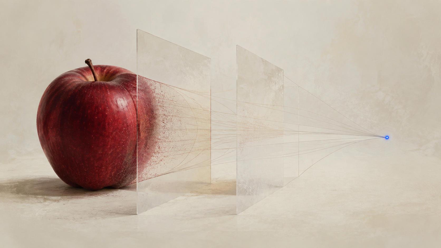
An apple sits on the table.
You pick it up, wondering whether it is sweet. The fruit seller puts it on a scale, working out what to charge. An artist moves it toward the window to see how the light falls on its skin.
Everyone is looking at the same apple, but each is looking for a different answer.
Put the apple on a digital scale, and it will tell you neither which tree the apple came from nor whether it will crunch when you bite into it. A reading appears on the screen: say, 180 grams.
That reading tells you something about the apple. It is far from everything.
There is something in school mathematics that does this sort of thing every day. We draw its graph, write down its formula, and study its maximum, minimum, and rate of change.
It is called a function.
Set the coordinate axes aside for a moment and think of a function as a way of observing. It begins to feel surprisingly natural. Follow this thought a little further, and a deeper question emerges: When we observe something, which relationships are we unwilling to lose?
01 · Turning a Question into a Function
A function is often written as
We can begin with a plain reading of this notation: give me an input from , and I will use the rule to produce one definite result in .
For weighing apples, could be the set of apple states we are considering, the possible readings on the scale, and the weighing rule. To keep instrument noise out of the discussion for now, we treat this as an idealized model under fixed conditions.
Then tells us what this observation returns when the apple is in state .
No elegant algebraic formula is required. Assigning a book its page count, a date its day of the week, or a photograph its black-and-white version can all be functions.
Each example does something similar: it uses a definite rule to represent an object through a particular result.
The same object can be observed in many ways. We can ask how much an apple weighs, which color category it belongs to, or simply whether it weighs more than 200 grams.
That last question needs only two possible answers: yes or no.
A function's output, then, need not be a number. It can be a category, an image, or a precisely defined yes or no. We decide what to ask, then choose the space of answers we need.
This is why thinking of functions as observations does more than give them a friendlier name. It shifts our attention from “How do I calculate this expression?” to “What does this rule make visible?”
Of course, functions can also describe actions and transformations, such as rotating an image ninety degrees. Observation is a useful way to understand functions; it does not exhaust what functions can mean.
02 · The Same Weight Does Not Mean the Same Apple
Now place a second apple on the table.
It may be redder, more sour, and from a different tree. But on the same scale, it too produces a reading of 180 grams.
Different apples, identical observations. In mathematical notation:
Once all you have left is that reading, you can no longer tell which apple was weighed.
This is where information is lost: two situations that could originally be distinguished have been merged in the record.
Imagine the function sorting all the objects into groups. Anything that produces the same observation goes into the same group. Weighing groups together apples that give the same reading. Asking only “Does it weigh more than 200 grams?” merges still more apples into just two groups: yes and no.
The coarser the observation, the more situations it may group together.
That does not make a coarse observation worthless. If you only want to select apples that meet a packaging weight limit, the instrument may have no need to report their color, variety, and sugar content as well.
For this task, those differences can be left out of the answer.
One qualification matters here: not every function merges different inputs. Take . If you know the rule, you can subtract 10 from the result and recover the original number. The identity function, , leaves the input exactly as it is.
So “Observations often discard detail” fits everyday experience. “Every function necessarily loses information” is not a mathematical fact.
Once we separate these claims, we can ask a better question: when an observation does discard detail, what makes that loss acceptable?
03 · A Map Can Leave a Great Deal Out
Think of a subway map inside a train carriage.
To make the routes legible, it straightens winding tracks and draws stretches of different lengths as roughly equal. Most of the city's buildings, trees, riverbanks, and side streets are missing.
If its job were to reproduce the city, it would clearly leave out too much.
But you have just boarded a train. What you actually want to know is: Where should I change lines? Can I reach my destination from there?
The omitted details make room for something else: the order of stations, the connections between lines, and the places where you can transfer. These stand out, making your question easier to answer.
The map's value depends on the questions it promises to answer.
Now ask a different question: How far away is the next station? Would walking be faster than taking the train?
The map that was sufficient a moment ago may no longer be sufficient. The distance information sacrificed to make transfers clearer has suddenly become what matters most.
The same simplification can be just right for one task and misleading for another.
This gives us a concrete test of whether an observation is enough: If two situations are recorded as the same result, do they still have the same answer to the question you care about?
Suppose two apples both give a reading of 180 grams, and your question is “Does the displayed reading exceed 200 grams?” The same reading is enough to support the same answer.
If your question is “Which apple is sweeter?”, the same weight reading offers no such guarantee.
We can make this test more precise. Let be the observation already made, and let be the question you want to answer next. If there is a rule such that
then the observation alone lets you work out the answer .
This short equation captures a practical meaning of “enough”: the original object is no longer at hand, but the record you kept still lets you complete the task.
Conversely, if two objects have the same -value but different -values, no rule acting only on that shared observation can always give the correct answer for both. The distinction you need was erased in the previous step.
04 · Can a Computer Hold a Real Number?
We make similar choices when recording numbers.
An instrument measures a quantity and displays 1.23. This often means we have retained only a certain precision. Under the same rounding rule, 1.231 and 1.234 may both be recorded as 1.23.
In the record, they are no longer distinguishable.
You might think: Why not add more decimal places?
Greater precision certainly helps. But there is a more fundamental boundary between “retaining more detail” and “representing every real number exactly.”
Any finite computer record can be written as a finite binary string. There are finitely many one-bit strings, finitely many two-bit strings, and so on. By sorting first by length and then by order within each length, we can put all finite strings on one infinite list.
In mathematics, we say they are countable.
The real numbers are uncountable. Even the real numbers between 0 and 1 cannot all be put on such a list.
Under a fixed interpretation rule, therefore, we cannot assign an exact, distinct representation to every real number—even if records may be arbitrarily long, provided each one is finite.
A possible misunderstanding is worth clearing up: does this mean that any number with an infinite decimal expansion cannot be represented exactly?
No. We can specify one-third exactly by writing “,” and we can specify exactly with a finite definition or program. Writing out every decimal digit of a number and specifying that number with a finite description are different things.
The actual limit is this: within a fixed system of finite descriptions, at most countably many real numbers can be specified exactly. Such a system cannot cover all real numbers.
Recording numbers at finite precision is a more familiar, concrete choice. It makes storage and computation practical, while leaving us with a question: will the discarded decimal places matter in the next step?
For example, consider rounding to the nearest integer. Round 0.4 and 0.4 separately, then add them, and you get . Add them first to get 0.8, then round, and you get 1.
The same two numbers. The same rounding rule. A different order of operations gives a different result.
Details dismissed as “unimportant decimal places” can add up to a carry. Now our concern extends beyond the precision of each recorded number: have we also preserved the way the numbers behave under operations?
05 · Values Can Change While Relationships Remain
Let us try three small experiments.
First experiment: add 10 to every number.
2 becomes 12, and 5 becomes 15.
The values change, but their order does not. Before, 2 was less than 5; afterward, 12 is still less than 15. Their distance is unchanged too: the difference was 3, and it is still 3.
This observation preserves order and distance.
But it does not preserve addition. Originally, . Add 10 to each of these three numbers, and does not equal 17.
Second experiment: multiply every number by 2.
2 becomes 4, and 5 becomes 10.
Order is still preserved, but the distance grows from 3 to 6. This time, however, addition is preserved: , exactly twice the original sum of 7.
“Add 10” and “multiply by 2” are both easy to undo, yet they treat different relationships differently.
This reveals a crucial distinction: whether we can recover the input from the output and whether a particular relationship is preserved are two different questions.
A fully reversible transformation may fail to preserve an operation you have specified. Conversely, an observation that discards a great deal of information may still preserve a useful structure.
Third experiment: record only whether an integer is odd or even.
This is an extremely coarse observation. 2, 100, and 1,000,000 all receive the same answer: even. The word “even” gives you almost no clue which integer you started with.
Yet if the question is “Will the sum of two integers be odd or even?”, their exact values are unnecessary.
Even plus even is even. Odd plus even is odd. Odd plus odd is even. The two observations alone determine which category the sum belongs to.
Integer addition thus has a corresponding rule of combination in the tiny answer space of “odd” and “even.”
Add the integers first, then observe their parity. Or observe their parities first, then combine them using that rule. The result is always the same.
This is what preserving an operation looks like:
Here is simply a symbol for the parity-combination rule we just described. The operations on the two sides need not look alike: on the left, we add integers; on the right, we combine parity classes. What matters is that both routes lead to the same answer.
Compare this with rounding. Both observations merge different inputs, but parity works consistently with its combination rule, while rounding does not always work with ordinary addition.
Knowing how much an observation loses is therefore not enough to tell us how useful it is. We also need to know what we intend to do next, and whether the relationships those operations require have survived.
06 · What You Choose to Preserve Shapes the Mathematics You Do
By now, the abstract-sounding word “structure” has several concrete meanings.
It can mean order: which element is no greater than which.
It can mean distance: how far apart two positions are.
It can mean an operation: how two elements combine to produce a third.
The same real numbers, equipped with an order, form one kind of mathematical object. Equipped with a distance, they form another. Equipped with addition, they offer another set of questions.
The observations we allow will change accordingly.
To study order, we might require maps to preserve it: whenever , we must also have . An existing distinction may collapse to equality, but the order must not reverse.
To preserve distance exactly, we require the distance between any two points to remain the same after mapping.
To preserve addition, we require that adding first and then mapping gives the same result as mapping each input first and then adding.
These requirements select different maps. “Add 10” passes the first two tests but fails the third. “Multiply by 2” passes the first and third but fails the second.
This is where category theory begins to enter the picture.
In these examples, we first choose a class of objects with some structure, then choose the maps we allow between them. We might study partially ordered sets and order-preserving maps, or groups and group homomorphisms.
These maps must also be composable. If one allowed step takes us from to , and another from to , putting them together must give an allowed map from to .
This fits our experience of observation. First weigh an apple, then decide whether it exceeds a weight limit. Together, these steps still form an observation from apples to “yes” or “no.”
Mathematics also requires an identity map for every object, leaving it unchanged. And when we compose three steps, the final result must not depend on which two we group together first.
Objects, arrows between them, and composition satisfying these rules form a category. Here, the arrows are the maps we have chosen to allow. In more general categories, arrows can mean other things; they need not be functions between sets.
The question “What category are you working in?” now has an approachable starting point:
What kinds of objects are you studying? What relationships do they carry? How are you allowed to move from one object to another? How must those relationships be treated along the way?
What you want to preserve does not, by itself, determine a unique category. But it strongly influences your choice of objects and arrows.
Require order to be preserved, and you get one collection of allowed maps. Require distance to be preserved, and that collection changes. Whether a transformation is allowed depends on the specific requirements you have chosen.
07 · Back to the Apple
Look again at the apple on the table.
180 grams is one piece of information about it. It leaves out most of the apple's details, but it may be enough to price it by weight. If you are choosing apples for jam, the same reading may no longer suffice.
We use observations like this every day: a photograph, a report card, a statistical indicator, a brief description of another person. They bring certain aspects into view while leaving other differences out of the record.
These real-world activities are often more complicated than a deterministic function. They involve noise, change, and disagreement. Still, functions give us a clear starting point for asking more precise questions.
Which different situations does this record group together? What judgments can it still support? When I compare, add, connect, or further process these results, do the original relationships still hold?
Sometimes we need a more detailed record. Sometimes we need a different observation. Sometimes we have already kept enough information, but have never made clear exactly what it is enough for.
A function becomes more than a rule for calculating on paper. It can also express a definite relationship between us and the things we encounter: through this rule, certain things come into view.
Category theory invites us to look further—to ask whether the things that come into view remain related in the ways we need.
The next time you turn something rich and complex into a number, an image, or a short description, perhaps pause for a moment:
What judgments do I want to make from this result? Which relationships must survive for those judgments to remain possible?
References and Notes
[1] Brendan Fong and David I. Spivak. Seven Sketches in Compositionality: An Invitation to Applied Category Theory. arXiv:1803.05316v3, 2018. The starting point for this essay's discussion of “maps as observations” and “preserving structure” comes from Chapter 1, §1.1, especially pages 1–2 of the main text. See also §1.3.2 for observation and composition. Book PDF.
The apple, map, and parity examples are developed here to explain these ideas. The argument about finite descriptions of real numbers supplements the book's rounding example. Throughout this essay, “information loss” means that different inputs become indistinguishable in the record; no probability distribution or information entropy is introduced.
The cover is an AI-assisted conceptual illustration.
Appendix: The Mathematical Structure of Observation
The main essay approaches functions as observations through apples, maps, and numerical records. This appendix develops that perspective through mathematical definitions and propositions. Each section identifies the part of the essay it expands on. The proofs use only basic facts about sets, functions, and operations.
Conventions. We begin with deterministic observations: functions between sets. Here, “information” means the ability to distinguish inputs, not Shannon information. To avoid irrelevant issues involving readings that never occur, we often restrict a function's codomain to its actual image.
A · The Indistinguishability Relation Induced by an Observation
Expands Sections 01–02: how can two different apples become the same case under an observation?
Let be a set of states and an observation. Define
This is an equivalence relation: reflexivity, symmetry, and transitivity follow directly from the corresponding properties of equality. Its equivalence classes are
Thus collects all states that produce the same reading as . It is also the fiber of through , namely .
Let denote the quotient set of these equivalence classes, and define the quotient map
Proposition A.1. Every observation factors into “merge indistinguishable states, then label the resulting classes.”
More precisely, the map
is a bijection, and
where is the inclusion map.
Proof. All representatives of an equivalence class have the same -value, so is well-defined. If two equivalence classes have the same image under , their representatives are related by , so the classes are equal. Thus is injective. Every equals for some , so is surjective. The factorization holds pointwise. □
This factorization separates what is lost from how the results are labeled. Distinct states are merged at the step; simply relabels the equivalence classes with the actual readings.
Corollary A.2. Every input can be recovered exactly from its actual reading if and only if is injective.
Here, “recovered” means that there is a function such that for every . If such an exists, then implies . Conversely, if is injective, define ; injectivity makes this unambiguous. □
Connection to the essay. Two apples that both give a reading of 180 grams belong to the same fiber. Saying that the weight record cannot distinguish them means precisely that this fiber contains more than one state. By contrast, is injective: the values change, but the ability to distinguish inputs is fully preserved.
B · Exactly When an Observation Is Enough to Answer a Question
Expands Section 03: when is a map or a reading sufficient?
Let represent the question we actually want to answer. Its value may be a number, a category, or a truth value.
Definition B.1. An observation is sufficient for a question if there exists such that
This is a factorization of through . Observe first, then process the result, and you obtain the answer to the question.
We define on the actual image . There is no need to make it handle readings that never occur. Whenever we write below, we implicitly restrict the codomain of to .
Theorem B.2. The following conditions are equivalent:
- is sufficient for .
- is constant on every fiber of ; that is,
When these conditions hold, is unique on .
Proof. If , equal -values remain equal after applying .
Conversely, for , define , where satisfies . Condition 2 ensures that every such gives the same -value, so is well-defined. By construction, . Any satisfying this equation must take the value at each , proving uniqueness. □
Using the relations from Section A, condition 2 can also be written as
where equivalence relations are viewed as subsets of . In words: any states that merges must also be states that has no need to distinguish.
Connection to the essay. If the question is only “Does the displayed scale reading exceed 200 grams?”, then can be calculated from that reading, so is sufficient. If the question concerns sweetness, and two apples with the same reading have different sweetness levels, the theorem tells us directly that no subsequent rule using only the weight reading can answer the sweetness question correctly for every apple.
C · Observations Can Be Finer or Coarser
Expands Sections 02–03: how do we compare “recording more detail” and “recording less detail” precisely?
Fix a state set . For observations and , define
Read this as “ is at least as fine as .” Knowing the result of always lets us calculate the result of .
By Theorem B.2,
Notice the direction of inclusion: a finer observation merges fewer states, so its indistinguishability relation is smaller.
This relation is a preorder. Every observation can be obtained from itself using the identity function, giving reflexivity. If and , then , giving transitivity.
It need not be antisymmetric on observation functions themselves. For example, on , the functions and are different, yet each can be calculated from the other.
More precisely, and if and only if . In this case there is a unique bijection between the actual images satisfying . The two observations retain exactly the same distinctions and merely label their results differently.
Identifying observations of this kind gives a partial order. It can also be described in terms of partitions of and their refinement order.
Connection to the essay. Exact weight determines rounded weight, which in turn supports certain coarse classifications. Such post-processing can preserve or merge existing fibers; it cannot split states that have already been merged. This is a precise, deterministic, set-theoretic version of “post-processing cannot increase distinguishability.” It requires neither probability nor information entropy.
D · When Can Operations Be Performed on Observations?
Expands Sections 04–05: why does parity work with addition, while rounding causes problems?
Suppose carries a binary operation
We want to define a binary operation on the actual readings such that
In other words, operating on the original objects and then observing should give the same answer as observing first and then operating on the results.
Theorem D.1. Such a exists if and only if is compatible with :
When exists, it is unique.
Proof. If exists, identical pairs of input readings must give identical results under , so compatibility holds.
Conversely, define
Compatibility ensures that changing the representatives and does not change the right-hand side, so is well-defined. Every pair of actual readings has the form , so the equation determines uniquely. □
An equivalence relation compatible with an operation is called a congruence relation. It allows us to define an operation on the quotient set:
Example D.2. Parity is a congruence for addition.
Take , , and . If and are both even, then
is also even. Addition therefore descends to parity classes, where it becomes addition modulo 2:
Example D.3. Integer rounding cannot support any “addition of readings” that works for all real inputs.
Specifically, take with . This fixes the rounding convention at half-integers. We have
But
Both input pairs give the same readings, , yet adding first and then observing gives 0 in one case and 1 in the other. If a function satisfied for all , then would have to equal both 0 and 1—a contradiction.
Connection to the essay. The main text shows that rounding does not preserve ordinary addition. Here we prove something stronger: if we retain only the two integer readings, no alternative binary operation on the output side can repair the problem exactly for all inputs. To calculate the rounded value of the original sum correctly, we must retain more information or restrict the allowed inputs.
E · Reversibility and Structure Preservation Are Different Requirements
Expands Section 05: why can adding 10 be undone even though it does not preserve ordinary addition?
Given operations and , a function preserves these operations if
where . This is the equation from Section D written as an equality of functions. We also say that the corresponding square commutes.
Now take , with ordinary addition specified on both sides. For ,
whereas
Thus is an invertible function, but it is not a group homomorphism from the additive group to itself.
If we allow the output operation to change, however, the situation changes. Define
Then
Now is a group isomorphism. The identity element of the second group is 10, and the inverse of is .
More generally, if is a bijection, we can always transport an operation on to by defining
This automatically satisfies the operation-preservation equation. If is associative, so is : use to pull any three elements of back to , then apply the associativity of . Identity elements and other structure can be transported as well.
Connection to the essay. Saying “ does not preserve addition” assumes that ordinary addition has already been specified on both sides. This is perfectly consistent with being able to recover from . When discussing structure preservation, we must specify the structures on both the input and output sides. Section D goes further, identifying when even a noninjective observation allows a compatible operation to be defined on its outputs.
F · Organizing These Requirements into Categories
Expands Section 06: what else is needed to move from “what we want to preserve” to a category?
Definition F.1. A locally small category consists of the following data:
- A class of objects .
- For each pair of objects , a set of morphisms . If , we write .
- For every object , an identity morphism .
- For every triple of objects , a composition operation
These data satisfy associativity and the identity laws. For all composable ,
and for every ,
“Locally small” means only that the morphisms between any fixed pair of objects form a set; the objects as a whole need not form a set. All the examples below satisfy this condition.
| Category | Objects | Requirement on morphisms |
|---|---|---|
| Sets | Any function | |
| Partially ordered sets | implies | |
| Groups | ||
| Metric spaces | ||
| Metric spaces |
The names of the last two categories are notation adopted in this appendix. They use nonexpansive maps and distance-preserving maps as morphisms, respectively. The latter permits isometric embeddings; surjectivity is not required.
Why do these choices form categories? Because identity functions satisfy each requirement, and the requirements are closed under composition. For example, if and both preserve order, then
If and are group homomorphisms, then
The composite of nonexpansive maps satisfies
For distance-preserving maps, replace the inequalities with equalities. Associativity and the identity laws are inherited from function composition.
This also explains why simply choosing some functions we like is not enough to form a category. For example, the translations on with do not include the identity function. They therefore cannot, as given, be all the morphisms of a category whose only object is .
Connection to the essay. Choosing a category means specifying objects, morphisms, and composition together. What we preserve constrains the morphisms, but we must still check identities and composition. Even with metric spaces as our objects, we may require distances to be preserved exactly or merely never to increase. These choices give different categories.
The morphisms in these examples happen to be functions. In a general category, morphisms are part of the defining data and need not admit a description in terms of how individual elements correspond. Thus “all morphisms are lossy observations” cannot be treated as a general theorem of category theory.
G · The Universal Property of a Quotient Map: Expressing “Enough” Categorically
Expands Sections 02, 03, and 06: how do indistinguishability, factorization, and categories come together?
Return to an observation . Let
and define the projections by taking the first and second components of each ordered pair.
The quotient map satisfies
because a pair of indistinguishable states is sent to the same equivalence class.
Moreover, for any set and function satisfying
there is a unique function such that
To prove this, simply define . The preceding equality makes this well-defined, and the surjectivity of gives uniqueness. This is Theorem B.2 rewritten in terms of the quotient set.
In , this property says that is a coequalizer of and .
The terminology expresses something concrete. We require the state pairs listed in to be treated as identical, and performs those identifications. Any answer function that respects the same identifications factors uniquely through .
The “universal property” lies in the quantifiers: “for every and , there exists a unique .” It characterizes the quotient map by its relationship with all subsequent maps of this kind.
By Section A, is in bijection with , so , with its codomain restricted to its actual image, has the same coequalizer property. If we continue to regard as a function into all of and is not surjective, we cannot make this assertion: readings that never occur may destroy the uniqueness of subsequent maps.
Connection to the essay. In Section B, “What can we still answer from the observation alone?” led to a criterion about functions. Here it becomes a categorical universal property. Category theory expresses the quantifiers, composition, and uniqueness of the same mechanism in a unified language.
H · Why Finite Descriptions Cannot Cover All Real Numbers
Expands Section 04: making “we cannot store all real numbers” into a precise cardinality statement.
The set of finite binary strings is
There are exactly strings of length . Ordering first by length and then lexicographically lists all finite strings in a countable sequence.
Let be the codes allowed by a fixed representation system, with a decoding rule
We do not require this rule to be computable; we require only that each valid code specify one definite real number. Since is at most countable, its image is also at most countable. Cantor's uncountability theorem tells us that is uncountable, so cannot be surjective.
It follows that, in any fixed system of finite representations, uncountably many real numbers remain without an exact representation.
Allowing expressions such as “,” “,” or “” does not change the conclusion: these symbols and their finite definitions are still finite strings. They specify certain numbers exactly, but cannot cover all real numbers.
Connection to the essay. This result concerns which numbers a representation system can cover. A particular rounding function concerns how numerical inputs are merged into readings of finite precision. The former is a cardinality constraint; the latter can be analyzed using the fibers of Section A and the compatibility condition of Section D. They are related, but they are different statements.
A Guide from the Essay to the Appendix
| Question in the essay | Mathematical formulation in the appendix |
|---|---|
| Which states become indistinguishable under observation? | Fibers, equivalence relations, and quotient sets (A) |
| Is the record sufficient? | The target function is constant on fibers; factorization (B) |
| Which observation is finer? | The post-processing preorder and partition refinement (C) |
| Can we still perform operations on the observations? | Congruence relations and operations descending to quotients (D) |
| Why does reversibility not guarantee structure preservation? | Specified operations on both sides and transport of structure (E) |
| How do these requirements define a mathematical setting? | Objects, morphisms, identities, and composition in a category (F) |
| How does category theory express answering from the record alone? | The coequalizer universal property of a quotient map (G) |
| Why can finite descriptions not cover all real numbers? | Countability of finite strings (H) |
This appendix starts from the observation perspective in Chapter 1 of Fong and Spivak's Seven Sketches in Compositionality, cited above, and adds standard arguments from set theory, algebra, and category theory. Its organization and proofs were developed as mathematical supplements to this essay; they are not a paragraph-by-paragraph translation of the book.